
Using Simulations to Train And Test Machine Learning Applications
Generating high-quality training and testing data Machine Learning algorithms using simulations

Dominik Schröck
18.3.2019
An overview of how to monitor long-standing simulations and use the data for machine learning purposes
One of the challenges in training and testing ML algorithms is to obtain high-quality data: the live data your algorithms will be working on often is not available from the word go and even if it is, it may not contain all the features you want to train your algorithm on.
One approach to dealing with this is to generate data using simulations – this gives you full control of both of the features contained within the data and also the volume and frequency of the data.
In this post we show you how to monitor long-standing simulations and use the data for machine learning purposes without having to deploy on your own hardware – and with the use of as little code as possible! This example makes use of simulation data generated using our own BPTK-Py Framework. We employ various Amazon Web Services applications for focusing on Analytics and ML rather than code and hardware/software.
The Challenge
Writing Computational Essays Based on Simulation Models, you learned how we developed a Python-based simulation engine for System Dynamics and Agent-Based Modeling. It allows you to run complex simulations within the Jupyter environment and access the simulation results for further analysis.
Machine Learning (ML) algorithms are becoming part of our everyday life. Ad owners improve their targeting using the web surfing behavior of potential customers. Businesses use more and more data sources – both internal and external – to forecast future sales and modify their strategy, all supported by ML. Manufacturers want to predict machine performance and faults to reduce production downtimes or even accidents.
The choice of the right Machine Learning algorithm is hard. It requires a lot of real-world data and testing. But the availability of such data is not always given. Someone in the sales department might be able to give you sales data for last year. But who’s got those market research? Can you get access to the raw website analytics data? You might need those data on a click-stream level. But the DWH might only store them preprocessed as minutely data – or enriched with other – for your problem – useless information.
With BPTK you can develop models and rapidly test them. What if we combine simulation and rapid prototyping of machine learning algorithms? This way, you avoid the never-ending search for real-world data. With this approach you can:
- Simulate near real-world data
- Test different ML algorithms for solving your problem
- Learn which data sources help solve your problem
- Present your learnings to decision-makers and prove the advantages of using ML methods in your business context
In the following, we would like to present you with a little example of how we made use of agent-based modeling for a few ML use cases.
Amazon Web Services (AWS)
Amazon Web Services (AWS) is a powerful service for deploying scalable online compute and storage services. AWS maintains the hardware and software which means you can deploy data pipelines only with a few clicks.
Why we used AWS in this showcase? Because it allows us to concentrate on Machine Learning algorithms and methods rather than wiring up infrastructure and writing big amounts of code before even being able to test ML. We will go into more detail about the specific services we used later in this blog post.
The Simulation Model
We employ a simulation of an electric car. This is a classical IoT (Internet of things) use case. Nowadays, cars are constantly sending statistics to the manufacturers’ servers in order to help improve the product. The data are processed in real-time. In the simulation, each car acts as an agent and has a battery. We did not model an engine or any other components to keep the model as simple as possible. Let us quickly go over the simulation models and the variables we measure. Figure 1 illustrates the states of the car we are going to work with.

Figure 1: State chart for car battery simulation
In each simulation round, the car either drives, charges or the battery is replaced. The battery might be failing. On battery fault, it takes one more simulation time step to replace the battery. In this simple model, a battery fails if its capacity falls below 14,000 amp, with a design capacity of 20,000 amp. The capacity reduces with every round due to driving and recharging, just like in the real world. Battery states are stored in the “battery state” field. On driving, the car uses 39.7 amp per kilometer, resulting in around 500 km per full charge (when the full capacity is still available). The number of kilometers driven in a simulation time step is a random value within certain bounds, given by a driving strategy. The replacement will only occur if the battery entered the failed state before. Whenever the car drives, the field “distance in period” stores the km driven within the given simulation period. It defaults to zero when charging. The field “charge”‘ measures the current charge of the battery. The “cycles” field increases by one on a full recharge. The car charges if a lower bound of charge has been reached. This lower bound is as well defined by the strategy.
The selection of the strategy is random at model initialization. We define three driving strategies:

In this article, we focus on the battery’s capacity. The capacity determines if the battery has to be replaced. It would be great to be able to forecast this value. Hence, we should have a look at the battery’s capacity over time for one agent. Check out Figure 2 for the results of a simulation that ran for 100,000 steps. We clearly see a rather simple pattern: The capacity starts at 20,000 amp and – almost linearly – decreases to 14,000 before the battery is replaced and the pattern restarts. If you’d look more closely at one cycle, you’d notice that the capacity decrease is not really linear. This is due to the fact that the car drives certain kilometers within the strategy’s bounds and not a fixed number of kilometers in each timestep. However, one could easily construct a function to estimate a battery fault event.

Figure 2: Battery capacity over time for the car simulation. Steps: 100,000
This model may be quite simple but good enough for our purposes in order to test methods for forecasting battery fault. In the real world, a prediction engine for battery fault is useful to inform the driver about making an appointment with the nearest workshop – before he breaks down in the middle of the road.
In order to forecast such problems, car manufacturers may employ data science techniques. A car could send its own telemetry data to the manufacturer’s servers, which uses a trained model based on millions of other cars. As a response, it may receive a warning if a battery fault in the near future is forecast.
Technologies Used in This Proof-of-Concept
Figure 3 depicts the structure of our machine learning framework used in this Proof-of-Concept. While the simulation may run in any Python environment, the rest of our data pipeline is processed by various Amazon Web Services applications. For large-scale simulation jobs, we employ an EC2 instance. The following sections go over this AWS pipeline and the technologies used.

Figure 3: Data pipeline
AWS Kinesis (Stream, Analytics, Firehose)
AWS Kinesis provides message queues or data streams. Each stream can have one or more producers and consumers. Producers push data while consumers pull them for further processing. Kinesis makes sure to distribute the data to all consumers and holds them until consumption. For computing aggregates, we employed Kinesis Analytics. This service accesses Kinesis streams and allows for SQL-like access to the data. As we deal with streaming data, which never ends, each query requires a window for processing aggregates. Windows are either count windows or time windows. A count window takes a fixed number of records, e.g. 1,000 records and computes an aggregate (AVG, MIN, MAX and so on). A time window on the other side collects the records of a defined time interval. Furthermore, a window can either be sliding or tumbling. A tumbling count window of 100 triggers whenever 100 events arrived. A sliding window of the same size triggers whenever a new event arrives and takes all the previous 99 elements of this particular event.
We implemented the following three queries to showcase the capabilities of Kinesis Analytics:
- Average kilometers driving per period in the last 10 periods: Quickly monitor the average kilometers each agent drives per period.
- An average number of kilometers until the battery fails in the last 1 hour: Monitor the number of kilometers until a battery fails. “1 hour” describes the time when the events arrived, not when they were generated in BPTK.
- Anomaly detection: Detect anomalies in the streaming data and measure them using an anomaly score.
The output of AWS Kinesis Analytics queries flows into another Kinesis Stream. These data are consumed by AWS Kinesis Firehose. Firehose is another component of Kinesis. It takes a Kinesis Stream as Input and outputs them in a structured way to other AWS applications. Using Firehose avoids coding your own stream consumer. It pushes the streaming data into the target applications without much configuration required. Here Firehose is used to output the data to S3, a scalable data storage – more on that in a later section.
AWS Lambda
For forecasting, we employ AWS Lambda. Lambda is a service that allows for executing arbitrary code – called a Function – whenever a trigger is executed. A function is stateless which means that all variables are lost after the execution finishes. The code is triggered whenever a condition applies. In this showcase, we use the Kinesis stream as a trigger. We configured Lambda to execute our function whenever 100 events arrived.
The function itself is a small Python script that receives the records, computes forecasts for each agent and fires the data out to another Kinesis stream. The virtual environment in which the code runs comes only with the most basic Python packages. Hence, you will have to download the Linux packages for all requirements and add them to the code package. Note that some packages such as numpy and pandas need to be compiled. We used an Amazon Linux VM and ran the following commands in a virtual environment:

Just copy the contents of the virtual environment’s site-packages into a zip file along with your function.py. Next, we copied the zip to an S3 bucket (S3 is a storage service provided by AWS) and configured the Lambda function to pull the file from the S3 location.
For forecasting the battery’s capacity, we employ Autoregressive modeling. This method creates a function that weights previous observations’ influence on future values. An alternative is the use of a moving average. Both methods are widely used for forecasting. Extensions such as ARIMA (combining both methods) are also common. For training the models, we use the python package statsmodels, an easy-to-use package for statistic modeling. The basic training and prediction code are pretty simple and straightforward. For a great example, check out this blog post.
Most of the code we had to write deals with decoding the incoming streaming data and preparing them for model training. The data structure is very intuitive. The lambda function receives a dictionary with a list named records. Each list element stores a dictionary named kinesis, which includes metadata for the given record and the raw data. Note that the data from a Kinesis stream arrive base64-decoded in a Lambda function. This is due to the fact that kinesis is agnostic of which type of data arrives. This means you need the base64 package to decode the JSON string. The function extracts the capacity field for each record and writes them into a list. The model fitting itself only requires few commands:

AWS S3
AWS Simple Storage Service or commonly referred to as “S3”, is a scalable online object store. It allows you to store any data which other applications consume. Data are organized in buckets. Each bucket can be configured separately, including access rights, visibility and read/write permissions. Each of our Firehose processes (one for each query) writes the result data into a different S3 bucket. S3 does not limit the storage you can use. You rather pay for what you use and how much you use it. This makes S3 scalable. Furthermore, it comes with high availability and performance. Just with all the other services, Amazon makes sure to provision hardware and software required to use the resources, without the need for your own physical hardware. Libraries for S3 are available for many programming languages. So even non-AWS applications can access the data from S3.
AWS Quicksight
The last tool in our chain is AWS Quicksight. Quicksight is a Business Intelligence tool that is able to connect to many data sources for graphical analysis. The front end is very intuitive and simple. For pulling data from S3, just click “Add Data Source” and select “S3”. Quicksight requires a JSON file that specifies the S3 bucket(s) and subfolders where it is supposed to pull the data from. Let us look at an example:

The URIPrefixes field sets the directory(ies) to search for data. Quicksight parses all entries and pulls all subfolders and files of the prefix. In the given example, it parses all files and subfolders within s3://the-bucket/subfolder/. The globalUploadSettings field contains information on the data. We instruct Quicksight to parse the found data as JSON files. After adding all data sources, we are able to create graphs and analyze the results.
Visualization And Analysis
Figure 4 shows the average number of kilometers each agent drove per period. Here we ran the simulation for four agents. We can easily identify two groups of agents with different driving behavior. The agents with the more aggressive driving strategies also drive more, while the conservative agents – of course – drive less. In a simulation with many agents, you can use the series data as input for training different clustering or classification algorithms.

Figure 4: Average kilometers per agent per period
Next is the anomaly score – a built-in function using Random Trees to detect anomalies within the received stream. You see the anomaly graph in Figure 5 for the first 50 simulation time steps. The bar chart on the left Y-Axis depicts the charge per time step. The line graph shows the anomaly score for each timestep. The anomaly is computed over all numeric fields the stream receives. The value hovers around 1, which is very small. This is not unexpected as the function does not show large anomalies. We observe a very clear pattern in the charge graph. It runs low until the agent recharges the battery. On every recharge, we observe a small peak in the anomaly score. The anomaly score is computed over a window that you can adjust in the query. You may use different window sizes to improve anomaly detection. A too-large window might lead to a very slow reaction to anomalies while a too-small window may result in many false positives as past observations with similar patterns are not taken into account.
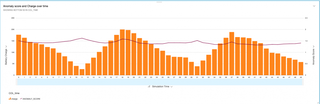
Figure 5: Anomaly score
Now let us have a look at the most interesting graph, the battery capacity forecast, which is available in Figure 6. We see how the forecast resembles the pattern of the actual capacity development. Obviously, the AR method is a good fit for this cycle. The algorithm always uses the last 100 observations to forecast the next 100 steps. The forecast was able to successfully predict the trend and we could use this as a warning for a battery fault. The numbers will not be 100% accurate, but a forecast does not necessarily have to meet the exact number but resemble the trend in order to allow for measures to avoid battery fault.
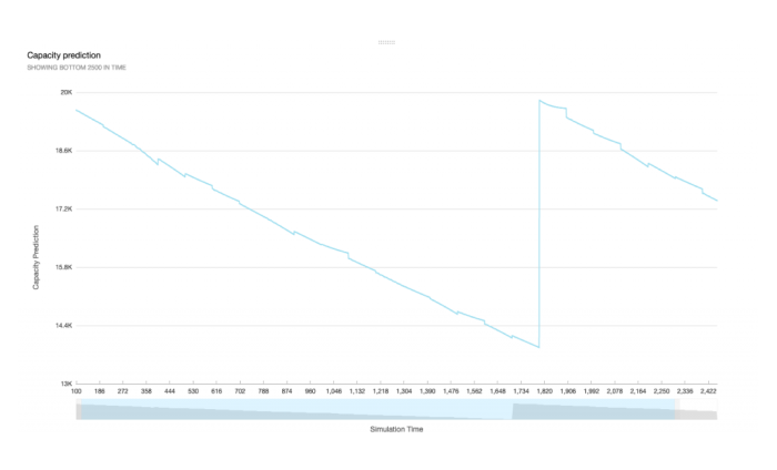
Figure 6: Forecast using an autoregressive Model, computed using AWS Lambda
Learnings
The goal of this proof-of-concept was to develop a scalable data intelligence application, using simulation data. This approach supports machine learning projects at an early stage where real-world data are scarce or hard to come by. With the use of cloud infrastructure, complex machine learning applications are easy to deploy. Thanks to the cloud, we could easily extend this with applications that consume the simulation data stream. Furthermore, we showed that using simulation data is useful for prototyping machine learning.
As a data scientist, I could now test other forecasting methods such as Moving Average, ARIMA or even deep learning using the same data we just generated in the simulation. And even test them side-by-side and compare the results within Quicksight.
We believe that at the early stages of Machine Learning/Data Science projects, simulation is able to support decision-making in regards to the choice of data sources, AI methods and budgeting.


Workshops
Resources
All Rights Reserved.