Infrastructure Simulation

An agent-based approach

Dominik Schröck
Tuesday, November 12, 2019

An investigation of own alternative approach using agent-based simulations and the BPTK-Py framework for modeling IT infrastructure simulations

Server and infrastructure sizing is a common problem in large IT projects. It usually ends with large, complex spreadsheets and many variables that in some way influence cost and resource utilization. For each project, you need to identify cost and resource drivers and define their influence on the overall system. This approach is tiresome and lacks the dynamics of system interaction and cannot cover a large set of different scenarios and their effects on the infrastructure.

In this blog post, we would like to demonstrate how we use our own Simulation framework for modeling IT infrastructure simulations. If you did not hear about the simulation framework yet, find info on

BPTK-PY

Writing Computational Essays Based on Simulation Models.

An IT infrastructure is a collection of systems that interact with each other – usually in the form of data flow. Each system has properties such as a maximum communication speed (e.g. 1 GBit/s for an ethernet interface) or memory/storage constraints.

To identify bottlenecks and estimate the real cost, we need a simulation that takes into account these constraints and the data flow within your infrastructure. With our approach, we model the infrastructure as a graph of systems. Edges denote the data flow, while nodes describe the systems involved (compute units, applications, data streams…).

With

BPTK-Py

, you can define such simulations easily. This is why we decided to predefine common systems in an infrastructure environment and make it easy for you to connect them.

For now, there are the following systems available:

Input: Data Stream of incoming elements, also called Source. Produces elements in a sinus function hovering around an average. The output is the data produced in MB
Kinesis Stream: AWS Kinesis stream that accepts an input and produces an output.
Target: Receiver of processed Events
Lambda: AWS Lambda function, mainly used for data transformation
Load Balancer: Distributes the incoming stream among computing units
Compute: These units process the data and output processed data to the Target(s). They have memory and storage. They receive incoming events and output a fixed number of events per timestep. They may also reject data if memory and storage run full.
Query: Pull data regularly from another system, e.g. another Compute unit that represents a database

Targets, Load Balancers and Compute have queues (in Compute this is storage and memory). If the queues run full, they will reject data and return it to the sender. The events are then added to the receiving agent or rejected and propagated back to the previous agent. This allows us to identify possible bottlenecks and react.

To model the infrastructure, we created a very simple language that allows you to create models like this:

Infrastructure Model designed in Enterprise Architect

The Simulation Model

You can describe your model in YAML files and our framework is doing the rest.

In this simulation, each timestep represents one second. This way we are able to simulate the most accurate cost and performance figures. However, simulations might last quite long.

Let us start defining our simulation model. The first step is to create the model YAML file containing the main properties and 1 scenario.

Model:
  name : Infrastructure

The model starts with the Model declaration. Each simulation scenario uses this model. Next, we give this model a name, “Infrastructure”.

Now we can start defining our first scenario. The basic properties are the start time, duration and step size (dt). We open a list

scenarios

and add the scenario Job1:

scenarios:
     - Job1:
        starttime : 0
        duration: 3600
        dt : 1

Scenarios run independently from each other. This way, you can compare the results from different configurations with each other.

Now we want to add nodes. The following lines add the nodes for two data pipelines that run alongside each other:

nodes:
          - INPUT:
              type : data_input
              count : 1
              step : 1
              target : STREAM
              average_output : 80
          - STREAM:
              count : 1
              step : 1
              type: kinesis
              previous: INPUT
              target: LOADBALANCER
              cost_shard_hour : 0.018
              average_output : 20
              shards : 80
              max_shards: 100
          - LOADBALANCER:
              count :  1
              type: load_balancer
              previous : STREAM
              target : COMPUTE
          - COMPUTE:
              count : 2
              step : 1
              previous : LOADBALANCER
              target: TARGET
              type : compute
          - TARGET:
              type : target
              count : 1
              step : 1
              previous: COMPUTE
              max_queue: 1000000
          - INPUT_2:
              type: data_input
              target : STREAM_2
          - STREAM_2:
              type: kinesis
              target: LAMBDA
              previous: INPUT_2
          - LAMBDA:
              type: lambda_function
              target: DATABASE
              previous: STREAM_2
          - DATABASE:
              type: compute
              storage_size: 1048576
              previous: LAMBDA
              target: QUERY
          - QUERY:
              type: query
              previous: DATABASE

Look at the

type

declaration. This directive is available for preconfigured nodes with default configurations.

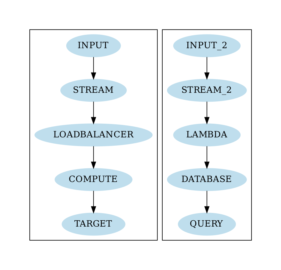
The first data pipeline is the one depicted in the above diagram. It comes with a Kinesis source, a load balancer, 2 compute units and one target agent. Note that the COMPUTE units’ count setting equals 2. This means the system group COMPUTE comprises a cluster of 2 virtual machines. The second pipeline simulates a distributed database that is fed by raw data delivered via a Kinesis stream. The preprocessing for the database is done with an AWS Lambda function.

The QUERY component simulates queries that run against the database cluster. In fact, we simulate the database as just another set of VMs that run one application, with bigger storage of 1 TB each. In fact, our simulation even supports simulating the storage’s read and write speed in MByte/s.

Both jobs run in the same scenario. This allows us the simulation of multiple pipelines that possibly interact with each other.

Each system comes with a predefined set of properties. You may override these, just as we did for

average_input

of the INPUT node for instance. The simulation produces an input resembling a sine wave, hovering around an average. Why? Because this allows us to simulate varying loads. We configured an average output of 80 MByte/s.

The options

previous

and

target

connect the nodes to each other. This way we construct the infrastructure as a graph, with data flowing from input to output.

The model is ready for simulation. Before we run the simulation, it is helpful to visualize the data pipeline as a graph. Let us quickly visualize the model before analyzing the simulation results:

Insfrastructure Simulation Blog post Graph 2

Running The Model

Now we are good to go and use standard functions from within

BPTK-PY

to run the infrastructure simulation. First, we are going to check out the Kinesis stream serving the input data to the data pipeline.

The Kinesis stream adjusts its number of shards in a given interval. One shard has a maximum input of 1 MB/s and an output of 2 MB/s. The standard setting for the property

reshard_interval

is 60 seconds. You can change this property as per your liking. For resharding, we use the average input to compute the number of shards:

shards = min( max( max_input, current shards), max_shards)

The

max_input

is the maximum input observed over the last

reshard_interval

periods. We set

max_shards

to 100 in the configuration (see above).

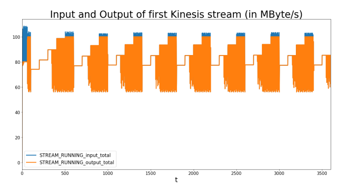
The following graph (by the way the graphs here are originally created with BPTK-Py) shows the number of shards and input/output per second in Mbytes. The input quickly increases, followed by a strong decline after which it hovers around 80 MB/s. This very much resembles the sine wave produced by the input. The input is always higher than the output because the number of shards is capped at 100, leading to a maximum input rate of 100 MB/s. Additional events get rejected and returned to the input. The input reacts to this and slows down. This leads to an equilibrium in the input and output of the Kinesis stream. The data input agent reacts by slowly increasing its output speed again until it worked off its queue and can send the data in almost real-time again. However, the Kinesis stream cannot pick up due to the shard constraint and has to reject events again, leading to a repetition of this pattern.

We can conclude that the maximum number of shards is a little too low for an optimal data flow. Whether this is acceptable, is of course always a business decision.

Now let us check out the other end of the pipeline, the

TARGET

system or application. We observe the same pattern as before, just with lower values. The reason is that the Kinesis units input/output ratio is set to 0.5, meaning that for every 1 MByte input, it outputs 0.5 MByte. Do not get confused: The measured numbers in the graph above show the number of processed bytes as compared to the input data to make the figures comparable.

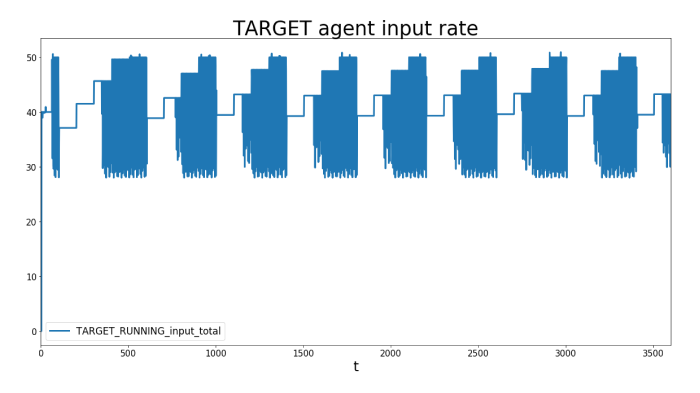
It is interesting to observe the dynamics of how the data pipeline adjusts its speed to the slowest element, which is the Kinesis stream in this case. Especially that pattern of the input source adjusting its speed regularly is interesting. Our goal is to increase the data output to the Targets’ maximum speed while maintaining the cost. You might want to reduce the number of computing units to a minimum in order to reduce cost. But keep in mind that in reality, you might want to guarantee redundancy. In this example, 1 rather than 2 compute units may be enough. On the other hand, we only simulated one hour. It might be exciting to run the simulation for a much longer time to see the effects on the VM’s storage and memory utilization. Especially, the distributed database in the second job might run full at some time, requiring another node to be added to the cluster.

Cost

After finding an optimal setup, it is time to analyze the cost factor, most important for business decisions for or against an infrastructure. Each node defines its own cost function and stores the cost incurred for each round. After improving the data pipeline and finding an optimal setup, we can have a look at the cost and cost drivers. An advantage of simulation as compared to static cost analysis using e.g. spreadsheets is that the cost resembles the dynamics of the overall system and its interactions. This system view allows you to find an optimal trade-off between cost and performance.

The following table shows each agents’ costs, followed by a sum after the whole 3,600 seconds for each agent.

And here comes the graph for the System components, with the total cost per second:

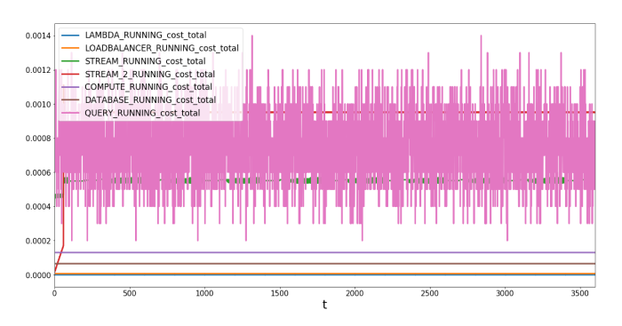
The cost for the QUERY system oscillates around 0.0009 US-$ per period. This is not surprising as it decides how often to query data against the database using a random uniformly distributed number.

We left out the input and target application, as we did not define any cost functions for them, leading to a constant cost of 0. You can however set the property

cost

directly to simulate constant cost and include it into your balance sheet calculations. Our reason for how these systems’ costs work is that they act as a dummy for any systems that are beyond the scope of this simulation. We just need their queue and other properties to simulate the data flow and identify bottlenecks. You can however set the

cost

property, resulting in a constant cost per round.

We observe the highest cost for the QUERY agents. This is due to the fact that we set a relatively high

cost_per_query

of 0.0001 $. You may reduce this by reconfiguring the job. The two kinesis streams are as well relatively expensive, with more than 5 USD for one hour.

Adding Complexity: Fail And Restart of Systems

In real-world environments, machines fail now and then. It is hard to properly simulate the effects of such scenarios using spreadsheets. We added specific model events, the

change_state

element. It can change a node’s state from one state to another. When triggered, it randomly selects one node that is in the target state from the target node group and changes the state.

It comes with 2 modes:

FIXED: Triggers at one specific time and changes one node’s state to the target state
RANDOM: Triggers in regular intervals and decides randomly upon its
```
likelihood
```
parameter whether to change states

Let us have a look at another simple example (shortened for improved reading):

Model:
       [...]
        nodes:
          - FAIL:
              type: change_state
              target : COMPUTE
              mode: FIXED
              trigger_at : 200
              state_map : {'RUNNING' : 'FAIL'}
          - RESTART:
              type: change_state
              target: COMPUTE
              mode: FIXED
              trigger_at: 2000
              state_map: {'FAIL': 'RUNNING'}
        [...]

In this scenario, we employ two new nodes:

RESTART

and

FAIL

, both being of a type

change_state

FAIL

will set one

COMPUTE

node’s state to

FAIL

at time 200.

RESTART

will do the opposite at the time 2000. The parameter

state_map

is important as it configures from which state to change to the target state. For instance, the

FAIL

selects one

COMPUTE

node that is in state RUNNING and changes it to FAIL.

Now we can play around with this example and analyze what happens before and after they fail. Let us have a look at the input/output rate of the COMPUTE units:

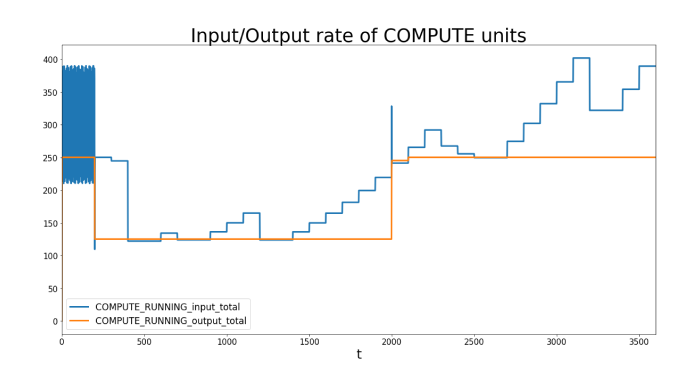
We observe a steady input/output rate up until time = 200 when one COMPUTE unit fails. However, the input still fires events, while the COMPUTE’s output reduces as only one is left, with a maximum output of 1GBit/s (125 Mbyte). After a while, the INPUT node reacts to the new situation and reduces its output rate as well, while it still tries to increase regularly. At time 2,000, the second COMPUTE unit is back to life, leading to an immediate increase in output rate to the maximum of 250 MByte/s.

The input stream however only increases its speed slowly in regular intervals and checks if it does receive rejection events before increasing more.

Conclusion

Modeling dynamic systems helps you simulate very complex interactions between elements of your environment and give you the insight you would never get when using static methods such as Excel. Simulation lets you easily identify bottlenecks, improve system performance and analyze the effects of edge cases like system crashes, before deployment. The result is a map of your future software and hardware environment.

This blog post demonstrated the abilities of our own Simulation Framework regarding Infrastructure simulations. Predefined systems as building blocks with changeable default configurations allow for easy model building. With our configurable approach, it is easy to design very complex data pipelines, without too much effort. This means you can concentrate on analysis and optimization, rather than model building.

In this little example we modeled:

Dynamic Rescaling of Kinesis Streams
Automatic adjustments of data rates of data pipelines using queues, similar to real-world behavior
Complex cost functions, including pretty accurate cost functions for AWS components
VMs with hardware constraints (HD read/write speed and memory)
Simulation of fail scenarios

COVID-19 And The SIR Model Overview Writing Computational Essays Based on Simulation Models